The great tidal earthquake hypothesis test, part III

Replicating and testing global studies of tidal earthquake triggering

Citation: Bradley, K., Hubbard, J., 2024. The great tidal earthquake hypothesis test, part III. Earthquake Insights, https://doi.org/10.62481/3b93879a

This is the third in a series of posts about whether earthquakes are influenced by tidal forces - and whether such influence might be able to tell us about upcoming large earthquakes.

In this post, we replicate aspects of three highly-cited studies on tidal triggering of global earthquakes to see whether previously found correlations still hold up. We also discuss some nitty-gritty details of the method, which turn out to be surprisingly important.

While we can replicate the methodologies pretty well, we do not find strong evidence for tidal triggering of global earthquakes in the new data. If a real correlation does exist between large earthquakes and tidal stresses, it must be an impressively small effect.

We encourage you to revisit our first post in this series, which explains some of the theory, and our second post, which summarizes these and other previous studies. In our next post, we will examine studies that explore variations in the sensitivity of large earthquakes to tides over time, in particular as a potential precursory signal to great earthquakes.

A quick note: Like in many of our posts, we are not experts in this field. We are learning as we go. We may get things wrong occasionally - so, at the end we provide our data, to allow checking of our calculations. If anyone identifies an error, we will happily update this post. We’ve appreciated the comments we’ve already received on some of the technical aspects of tidal triggering studies!

In our last post, we described and compared nine different studies that searched for evidence that large earthquakes are tidalific (to coin a term) - i.e., correlated with tidal stresses. What we found was that very few studies tried to replicate each other - and when they did, their results were often contradictory. Many of these studies are still cited as evidence for tidal triggering of large earthquakes, and as motivation for further research.

In this post, we turn our attention to the subset of those studies that proposed at least one positive correlation that has not already been directly contradicted by a later study. We want to know: how well do these studies hold up? There’s only one way to tell!

We also briefly revisit at a third study that has already been contradicted (at least in part), but where we previously did not understand one of their histograms. After all, this is an epic battle of histograms, right?

So in this post, we look at three papers:

Tanaka, S., Ohtake, M. and Sato, H., 2002. Evidence for tidal triggering of earthquakes as revealed from statistical analysis of global data. Journal of Geophysical Research: Solid Earth, 107(B10), pp.ESE-1. https://doi.org/10.1029/2001JB001577

Cochran, E.S., Vidale, J.E. and Tanaka, S., 2004. Earth tides can trigger shallow thrust fault earthquakes. Science, 306(5699), pp.1164-1166. https://doi.org/10.1126/science.1103961

Ide, S., Yabe, S. and Tanaka, Y., 2016. Earthquake potential revealed by tidal influence on earthquake size–frequency statistics. Nature Geoscience, 9(11), pp.834-837. https://doi.org/10.1038/ngeo2796

However, before we jump into the deep end of the pool, we need to discuss some technical aspects of the method (this is called diving into the shallow end of the pool).

If you want to skip the following section and go straight to the replication/testing, we just think it is important to keep these points in mind:

1. Tidal earthquake statistics are extremely sensitive to apparently minor details of how stresses and phases are estimated, and how data are selected.

2. The use of tidal phase as a statistical signal is fraught with peril - to the point that we aren’t sure it is very useful at all if the signals are not very strong.

3. It is very hard to look at subsets of global data without performing unintentional p-hacking.

Technical details I: The code we used

Most studies of tidal triggering significantly predate the practice of providing open code or data that could be used for validation. Thus, we had to rely on newer codes and similar, but not identical, data.

Fortunately, Hirose et al. (2019, 2022) recently published TidalStrain.2, a FORTRAN program that is the direct descendent of codes developed by Tsuruoka (1995), Tanaka et al. (2002), and others. Improvements in the code mean that we can try to bridge two worlds: replication of older studies using similar code, and calculation of hopefully meaningful numbers using an updated numerical approach.

While working with TidalStrain.2, we did make a few minor modifications to the code (which do not affect any published studies). We also validated our calculations against independently estimated ocean tides, and against tidal stresses calculated in other studies using other methods.

In the end, we used TidalStrain.2 to estimate six tidal parameters (ΔV, Δτ, Δσ, and ΔCFF at μ=0.1, 0.4, and 0.7), at both origin and centroid locations, for both nodal planes of each earthquake, for 63,720 events in the GCMT catalog, from January 1, 1976 through March 9, 2024. We also calculated τp (used by Cochran et al. (2004), discussed later.

Our computers sure kept the basement office warm for a few weeks! A good study to do during the winter months.

We have uploaded the resulting data files to GitHub so that anyone interested in this stuff can validate our validations, replicate our replications, or more deeply explore the data. We would definitely appreciate any feedback.

Technical details II: The problem with Schuster…

…is certainly not the dashing mutton chops he sported in his younger years.

Figure 1: In his later years, Schuster’s beard was more evenly distributed across his chin, with a p-value closer to 1. Is calculating the p-value of a beard distribution a purely new human thought? Let’s hope so.

Rather, the problem is with how his test is applied.

In our first post in this series, we described how a Schuster Test can be visualized as a zig-zaggy walk. (Interestingly, auto-correct tries to turn that word into zig-baggy… what is that?)

The p-value, calculated at the end of the walk, depends on the number of steps and the final distance from the starting point. This number can very sensitively indicate whether a bias exists in the walk direction: p-values close to 0 indicate the likely presence of a bias.

First, let’s look at a simple problem with the test, which could easily affect results in a very subtle way. The Schuster Test assumes a continuum of phases between -180° and 180°, but sometimes it is applied to data with integer phase values. This could be called the Discrete Schuster Test. Tidal phase is a truly continuous value, but phases are often estimated only to integer level. A quick test shows that you have to be very careful not to introduce rounding biases before applying the Schuster Test!

Figure 2: The impact of rounding on a p-value calculations for a dataset of 1,333 events. Left: Unrounded, p-value = 34.09%. Middle: Rounded to the nearest integer, p-value = 33.87%. Right: Rounded down, p=value = 23.61%. Note that in this case, the phase calculation remains unchanged.

But there is a second, and more interesting problem.

The primary assumption of the Schuster Test is that randomly timed earthquakes, when compared to tidal phase, will yield p-values close to 1, while even a subtle tidal triggering effect will cause a small bias detectable by a p-value close to 0 when enough earthquakes are included. The test is designed to find small biases in data.

Tidal phase is distributed equally between every tidal minimum and maximum (-180° to 0°), and between every tidal maximum and minimum (0° to +180°). But it turns out that tides often don’t go up and down at the same rate - so, they don’t spend the same amount of time going up as they do going down. This means that the time spent with phases <0° is different from the time spent with phases >0°. This is known as tidal asymmetry or tidal skewness.

If you search for tidal asymmetry on Google Scholar, you will find 138,000 results. Many studies deal with the movement of suspended sediments in oceans, rivers, and estuaries - the asymmetric tides are actually really important! Notably, it is now well understood that tidal asymmetry arises from purely astronomical effects as well as local effects like ocean currents.

To visualize this effect, we selected a location offshore of Noto, Japan, where the ocean tide is known to be asymmetric, and earthquakes are also abundant (like the M7.5 Noto earthquake that struck on January 1, 2024). We generated a 1-year time series of tidal ocean surface height using the OTPS software (tide model TPXO9.v2, starting at 2000-01-01). Stresses inside the Earth respond to this signal.

We then calculated the phase of the tide at 100,000 randomly selected times. Here is a histogram of the 100,000 phases:

Figure 3: Tidal phases of 100,000 randomly timed “earthquakes” applied to a tide curve near the Noto Peninsula, Japan. The plot shows the effect of tidal asymmetry on the spread of tidal phases. Note that this is the phase of sea surface elevation - not the stress on a fault - but the two are closely related.

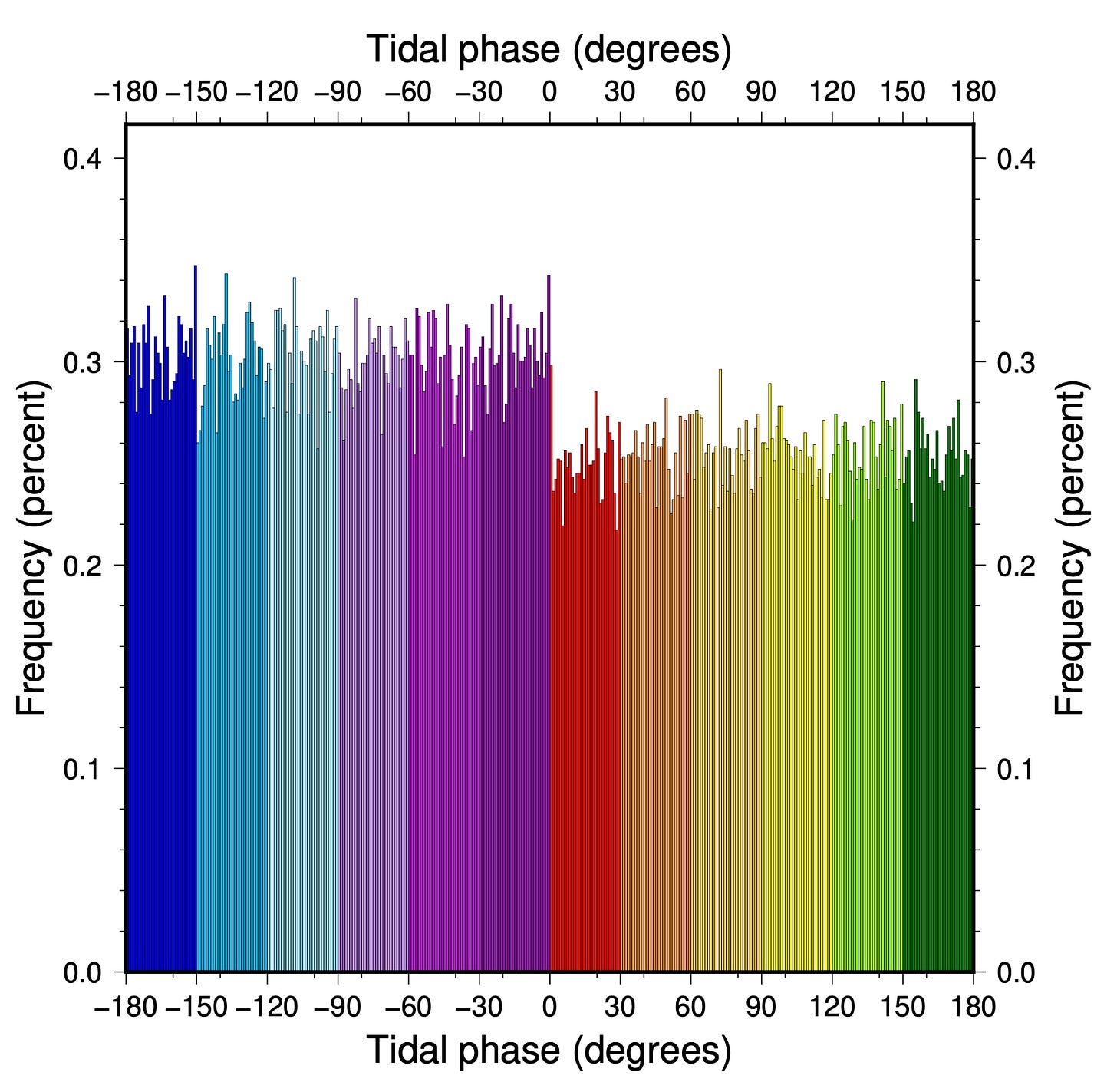
We can see that there are approximately 20% more events in each bin with phase < 0° than there are in each bin with phase > 0°, a feature that arises solely from the tidal asymmetry.

Could this affect p-values from the Schuster Test? We calculated tide height for three different time series: 19 years at 1 hour increments, 1 year at 5 minute increments, and 1 week at 5 minute increments. Then we randomly generated N “earthquakes”, measured their phases, and calculated the p-values of the “earthquake catalogs.” We started and ended the tidal curve at extrema to avoid biasing the results with a partial tidal cycle.

Figure 4: p-values calculated on the basis of N randomly timed events during a period of (left) 19 years; (middle) 1 year, and (right), 1 week.

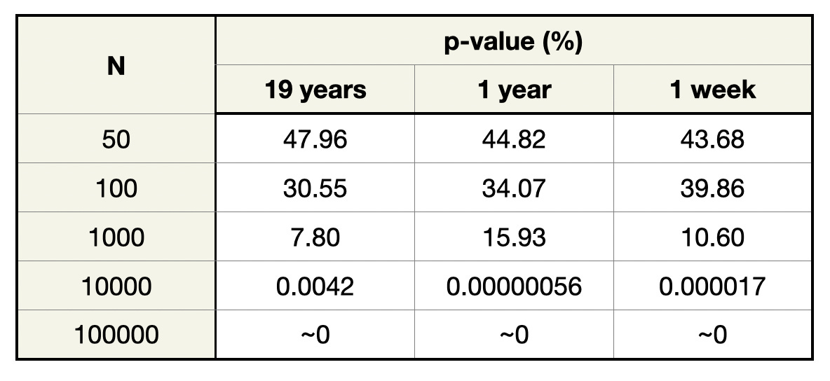
The results are clear. Random sampling in time produces in p-values well below 1. The effect becomes more extreme as the asymmetric tide is more thoroughly sampled.

This test reveals another thing about p-values: even when ~20% more earthquakes occur in positive than negative tidal phase, the p-value can be larger than 5% for N as large as 1000!

In most studies of tidally induced seismicity, tidal stress is estimated to influence 0-5% of earthquakes, which could only be detected with N well above 1000. So, we usually want to add earthquakes to our catalog if possible, to increase N. However, as N increases, the effect of biases like tidal asymmetry can begin to dominate the p-value.

Here’s a pretty map showing the asymmetry of the ocean tides, from Núñez et al. (2020), onto which we have overlaid the earthquakes in the GCMT catalog. It is clear that the tide is skewed to some degree, favoring either rising or falling tidal phases, over most of the oceans. The red earthquake zones traverse a varied landscape of tidal asymmetry. Different ‘types’ of earthquakes (subduction thrust events, mid-ocean ridge normal and strike-slip events, etc.) traverse different lobes of asymmetry. So, it is not easy to understand the possible effect of tidal asymmetry on a global catalog, or on particular subsets of the catalog - the effect will vary depending on the specific distribution of earthquakes.

Figure 5: Overlay of earthquakes from the GCMT catalog (red dots) on the map of tidal skewness in Earth’s oceans. Skewness map is figure 3a of Núñez et al. (2020).

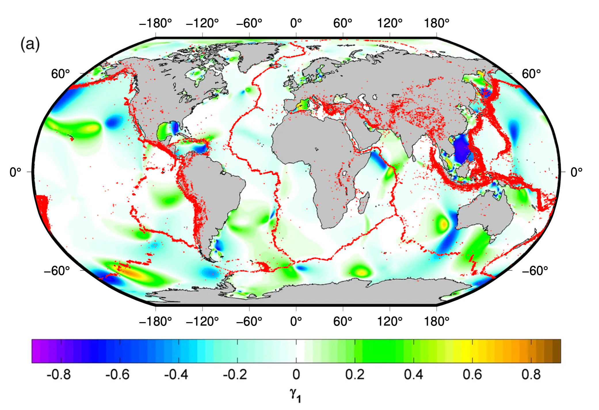
Is this asymmetry only a feature of the ocean tides, or does it also appear in the solid Earth tide? Examination of solid Earth tides calculated using SPOTL indicates an asymmetry of perhaps ~0.5%, at least in the one location we tested. We haven’t seen much discussion of body tide asymmetries in studies of tidal seismicity. It would be great to see someone pick this up as a research question!

These observations give us pause about the use of p-values from the Schuster Test for finding subtle correlations in tidal phase data.

The Schuster Test is the foundation of many of the studies we discussed in our second post, as well as several additional studies that we will introduce in later posts, and many studies that we don’t discuss. Its use has been called into question before, for other reasons, but we haven’t seen much discussion about the impact of tidal asymmetry. It would be really interesting to see a thorough analysis of this issue… hint… hint…

OK, let’s move forward with replication and testing of the prior studies. While we might be suspicious of the Schuster Test in general, many people do accept its utility, so we put aside our concerns for now and simply check whether prior results still hold up.

Let the histogram battle begin!

Replication and testing of Tanaka et al. (2002)

TL;DR: We replicate the original calculations of Tanaka et al. (2000) reasonably well. However, applying the method to the independent set of earthquakes since January 1, 2000 does not reveal the same correlations.

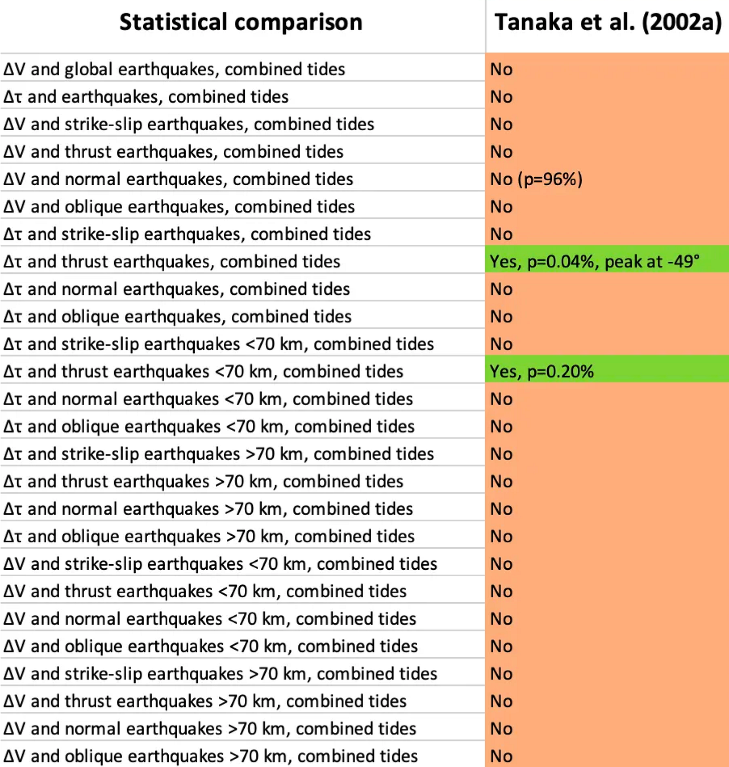
Tanaka et al. (2002) published the first really comprehensive survey of tidal triggering of large (M>5.5) global earthquakes. This paper is commonly cited as evidence that a special class of earthquakes - those occurring on shallow thrust faults - have a significant tidal signal. These particular earthquakes are important because they are a hazardous class of faults, and should be exposed to strong tidal stresses because they often occur underwater, near coastlines.

Recall ✨The Chart✨ from our second post:

Figure 6: Results of Schuster Test p-values for different statistical tests run by Tanaka et al. (2002). No = p-value>5%; Yes = p-value<1%. Peak indicates preferred phase.

Tanaka et al. used Harvard CMT earthquakes through the end of 1999, with stresses calculated at centroid locations. We instead used the GCMT database, which is the direct descendent of the Harvard CMT database (the name changed in 2006).

First, we validated our own calculations against the original publication. You can simply compare the gray histograms at left to the rainbow ones at right (Figures 7-12). You will probably find that the shapes, number of events, and sinusoidal fits are “pretty good”, all things considered. Don’t overlook our sinusoidal fit to the histograms (an unfortunately thin red line, at this scale)!

Figure 7: Validation of Figure 4 of Tanaka et al. (2002). Left: Figure 4 of Tanaka et al. (2002). Right: our replication. Recall that J1 is the same as ΔV.

Figure 8: Validation of Figure 5 of Tanaka et al. (2002). Left: Figure 5 of Tanaka et al. (2002). Right: our replication.

Figure 9: Validation of Figure 6 of Tanaka et al. (2002). Left: Figure 6 of Tanaka et al. (2002). Right: our replication. Recall that J1 is the same as ΔV.

Figure 10: Validation of Figure 7 of Tanaka et al. (2002). Top row: Part of Figure 7 of Tanaka et al. (2002). Bottom: our replication.

Figure 11: Validation of Figure 7 of Tanaka et al. (2002). Top row: Part of Figure 7 of Tanaka et al. (2002). Bottom: our replication. Recall that J1 is the same as ΔV.

Figure 12: Validation of Figures 8 and 9 of Tanaka et al. (2002). Left top: Figure 8 of Tanaka et al. (2002). Left bottom: Figure 9 of Tanaka et al. (2002). Right: our replication. Recall that J1 is the same as ΔV.

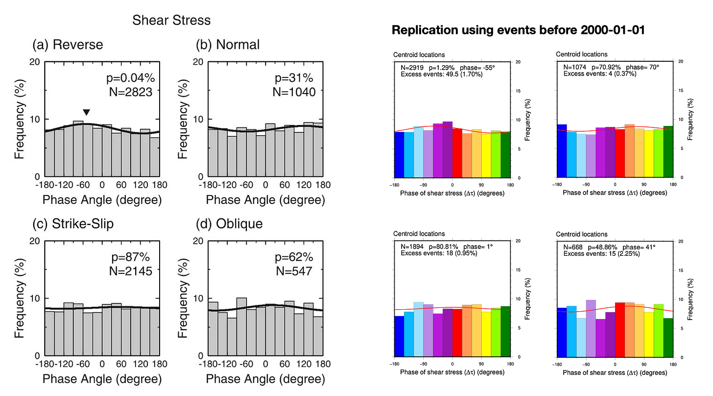
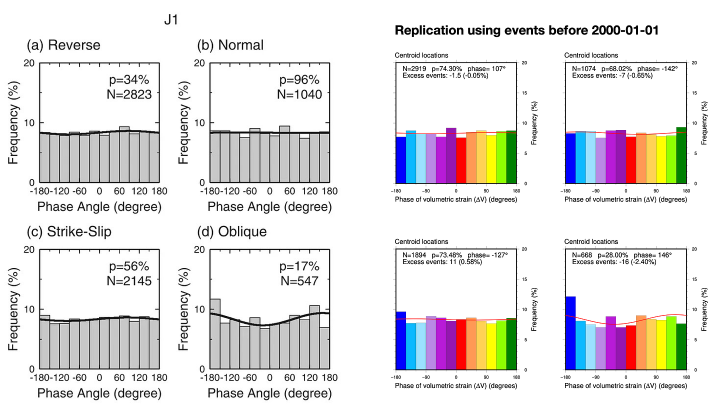
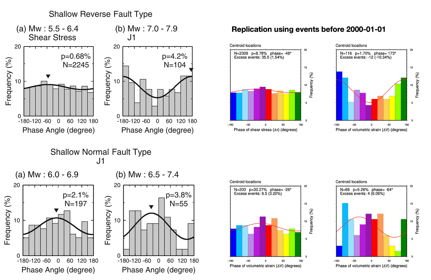
Overall, the replication is pretty good. The differences that exist likely arise from three sources:

1. Differences between the pre-2000 Harvard CMT catalog and the pre-2000 events in the current GCMT catalog,

2. Differences in the modeling of the tidal stresses using different codes, and/or

3. Differences in how tidal phases were extracted from the time series.

However, we think that the correspondence is good enough to say that we positively validate the calculations done in the original paper.

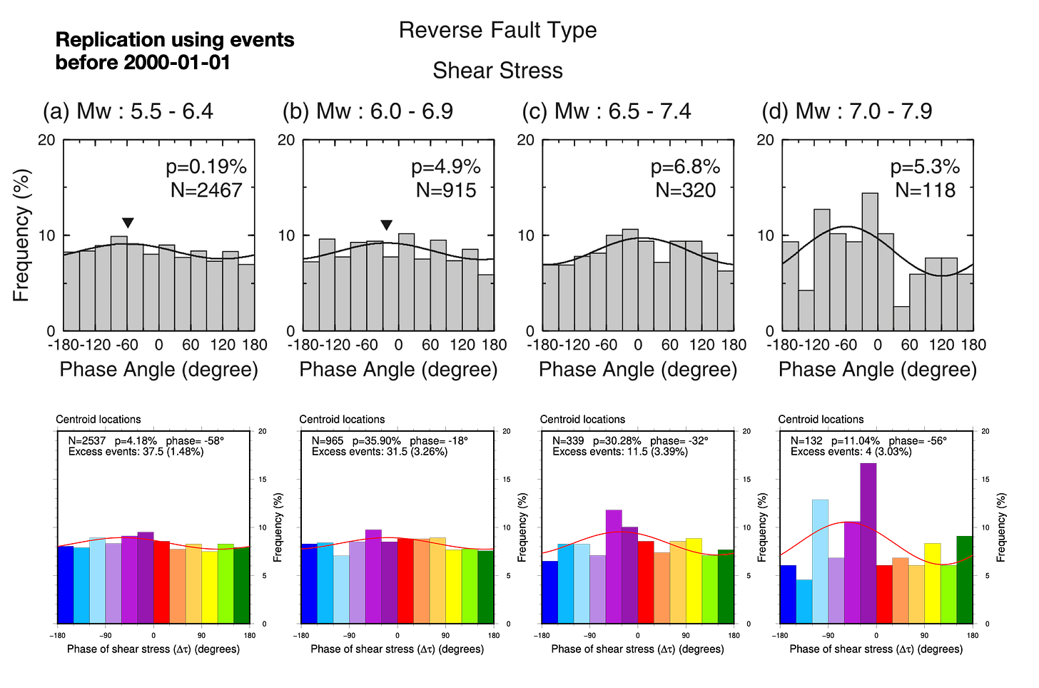
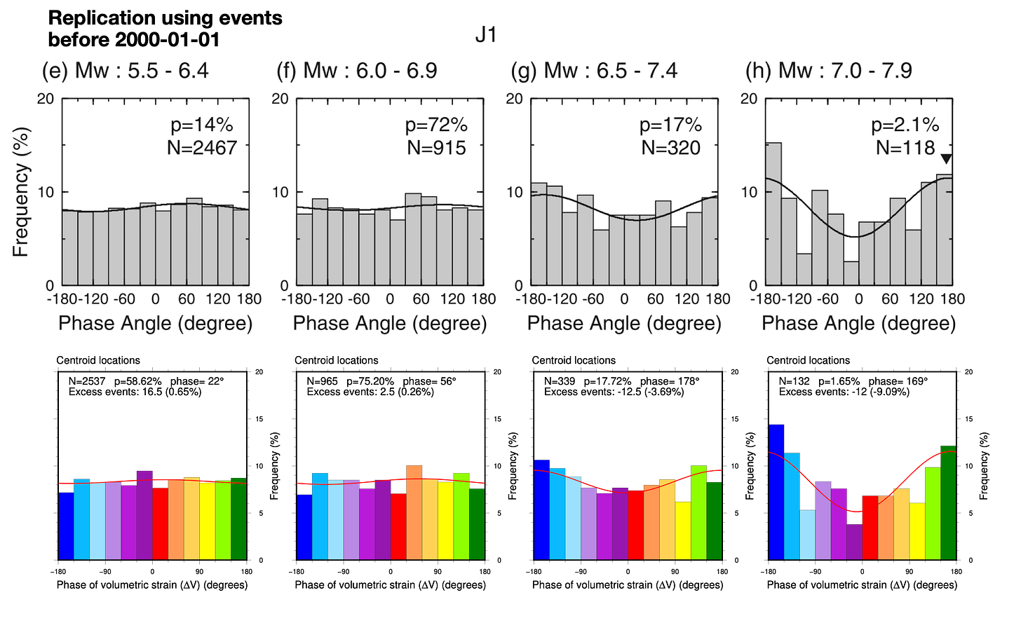
So, what happens when we look at the independent, post-2000 earthquake catalog (Figure 13-18)? The idea here is to check whether the histograms, p-values, and preferred phases (the sinusoidal fits to the histograms) are still “similar enough” to the original patterns.

Figure 13: Testing of Figure 4 of Tanaka et al. (2002). Left: Figure 4 of Tanaka et al. (2002). Right: our test using centroid locations since 2000-01-01. Recall that J1 is the same as ΔV.

Figure 14: Testing of Figure 5 of Tanaka et al. (2002). Left: Figure 5 of Tanaka et al. (2002). Right: our test using centroid locations since 2000-01-01.

Figure 15: Testing of Figure 6 of Tanaka et al. (2002). Left: Figure 6 of Tanaka et al. (2002). Right: our test using centroid locations since 2000-01-01. Recall that J1 is the same as ΔV.

Figure 16: Testing of Figure 7 of Tanaka et al. (2002). Top row: Part of Figure 7 of Tanaka et al. (2002). Bottom: our test using centroid locations since 2000-01-01.

Figure 17: Testing of Figure 7 of Tanaka et al. (2002). Top row: Part of Figure 7 of Tanaka et al. (2002). Bottom: our test using centroid locations since 2000-01-01. Recall that J1 is the same as ΔV.

Figure 18: Testing of Figures 8 and 9 of Tanaka et al. (2002). Top left: Figure 8 of Tanaka et al. (2002). Bottom left: Figure 9 of Tanaka et al. (2002). Right: our test using centroid locations since 2000-01-01. Recall that J1 is the same as ΔV.

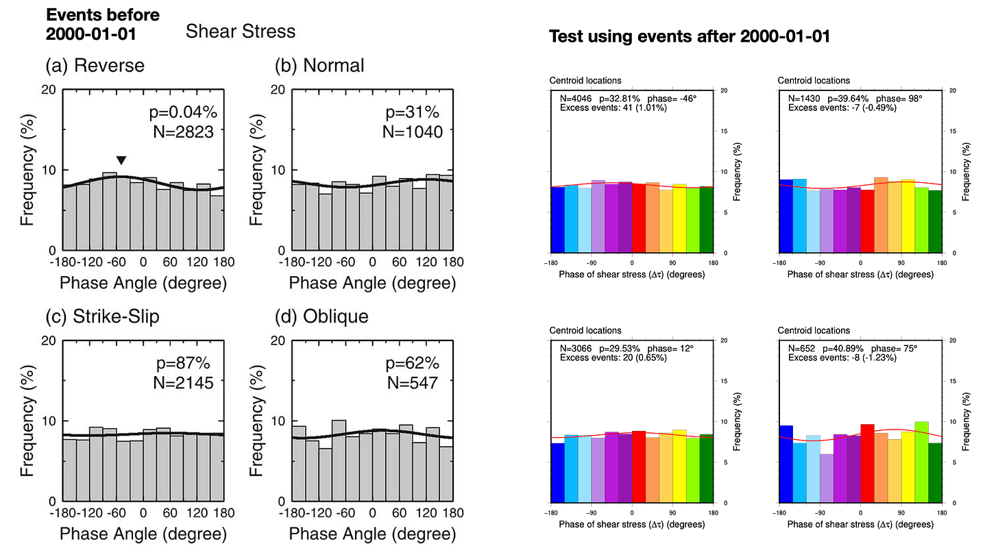
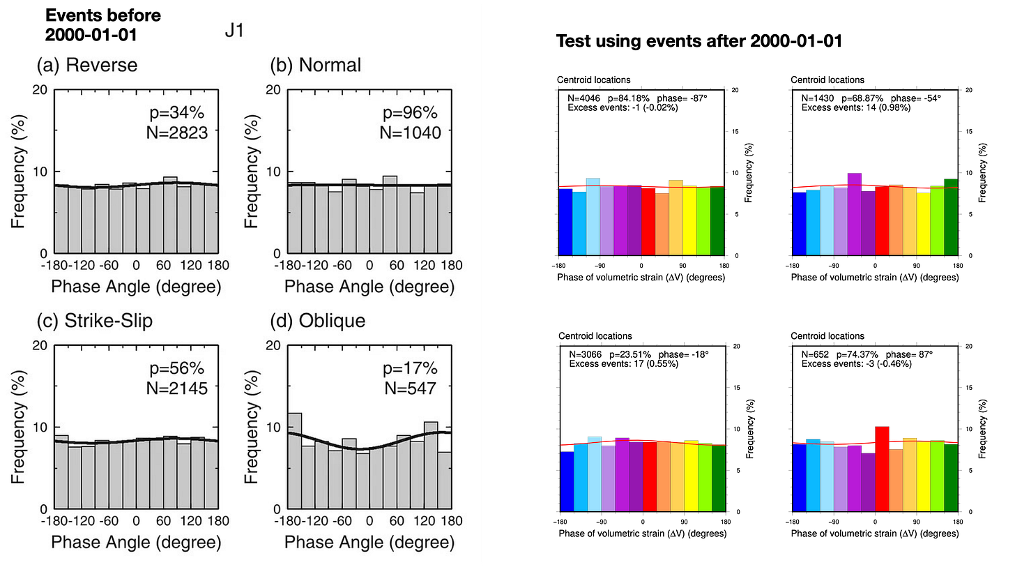
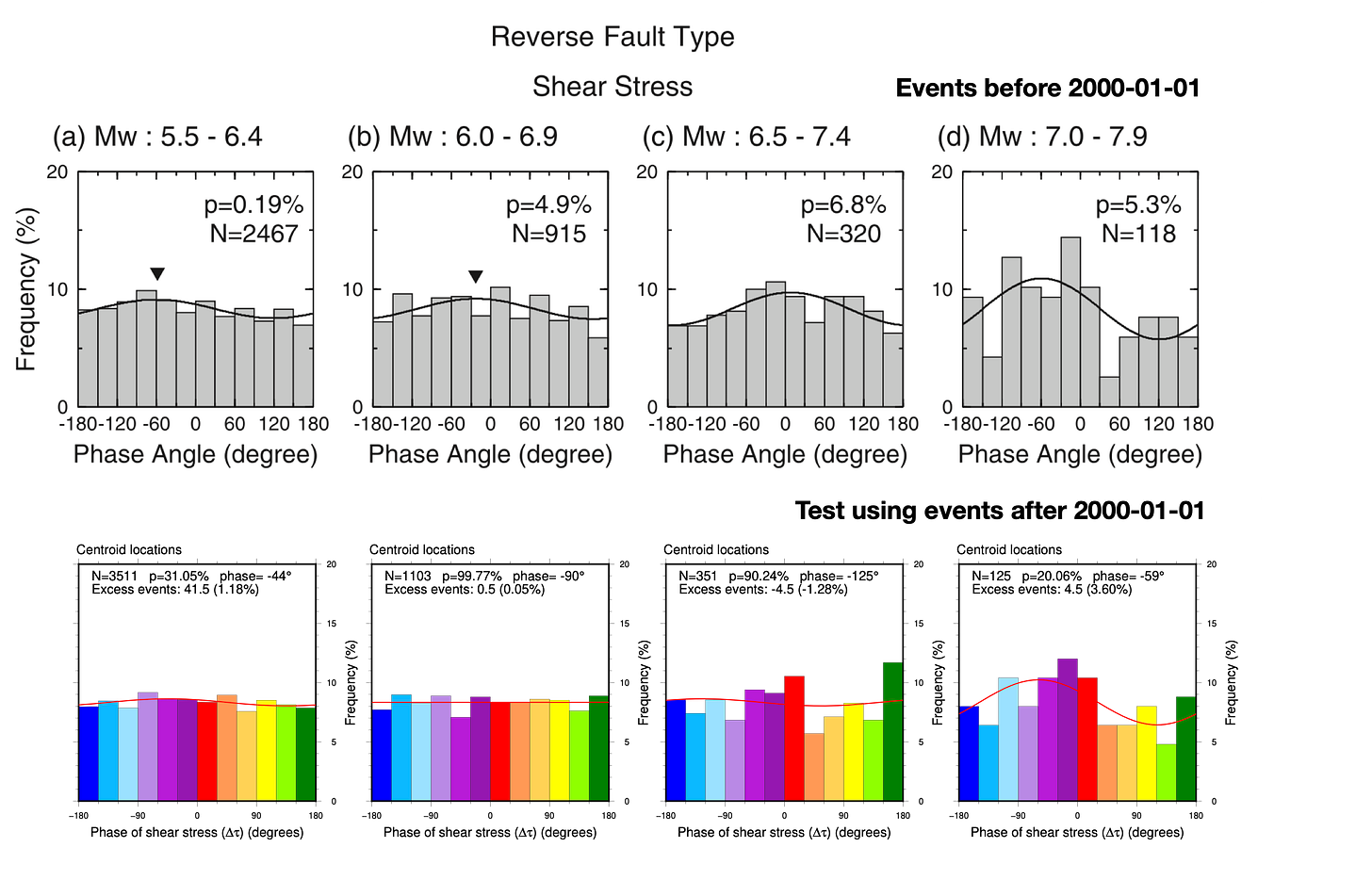
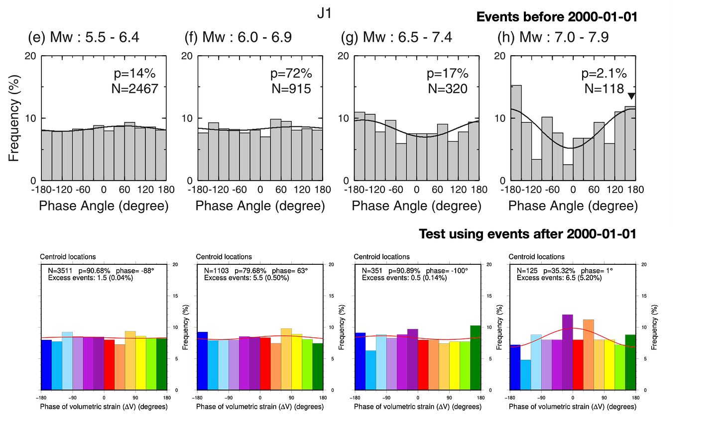
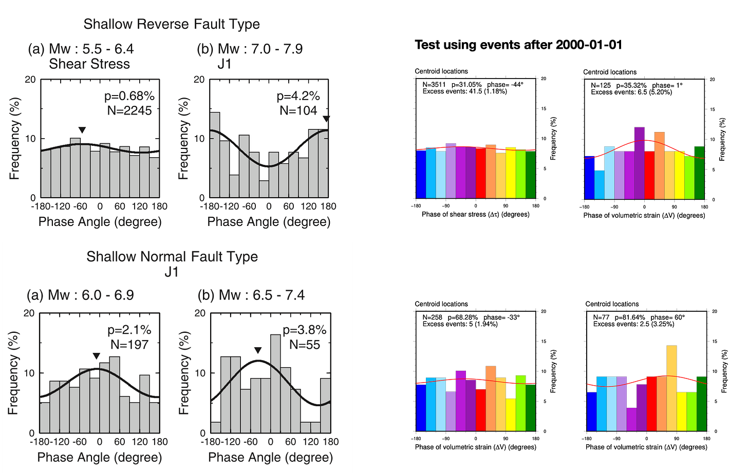
Most of the results are significantly different.

We summarize our replication and testing results in the following tables (Figure 19 and 20) - a veritable sea of p-values. Don’t spend too much time staring at the numbers - we will untangle the overall patterns below. For now, just know that any cell with a p-value below 1% is colored green (tidalicious); any cell with a p-value between 1-5% is colored yellow (tidalish); where p-values fall below 5%, we also indicate the preferred phase (Φ). Also, we apologize for reporting p-values to 0.01% - an implied precision far beyond reality.

The first table represents the content found in Tanaka et al.’s Figures 4, 5, and 6, plus our own validation and testing. For the testing, we also tried both centroid and origin locations, as well as a declustered origin catalog (“declustered” in this case means that we removed any event occurring within 24 hours and 300 km of a previous event, regardless of their magnitude - a pretty aggressive approach).

Figure 19: Summary of p-values from Figures 4, 5, and 6 of Tanaka et al. (2002), with our replication and testing. Replication was done using centroid locations. Testing results are shown for centroid locations, origin locations, and a “declustered” origin catalog, removing any event occurring within 24 hours and 300 km of a previous event.

The second table shows our replication and testing of Tanaka et al.’s Tables 2 and 3, along with a comparison between origins and centroids.

Figure 20: Summary of p-values from Tables 2 and 3 of Tanaka et al. (2002), with our replication and testing. Replication was done using centroid locations. Testing results are shown for centroid locations and origin locations.

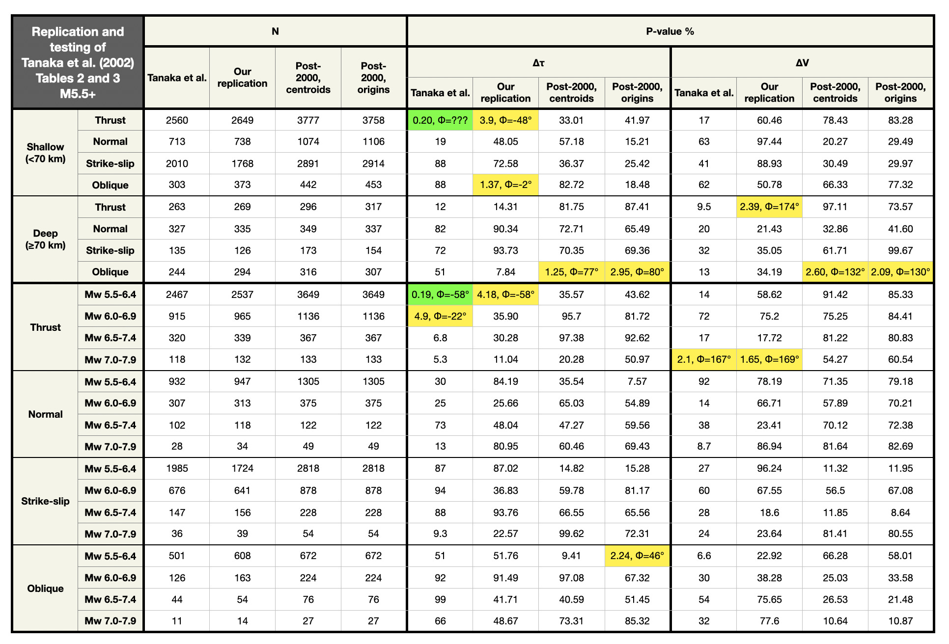
Basically, these tables show that:

• We replicate the results of the original study quite well, using GCMT data of the same time period.

• In no case was a low p-value for the pre-2000 dataset replicated in the post-2000 dataset.

• In no case was a low p-value for the post-2000 dataset found in the pre-2000 dataset.

• There are usually major differences between centroid and origin calculations.

• While we found a single p-value below 5% for the full dataset in the origins catalog, that p-value climbed above 5% when we declustered the catalog. Declustering usually changes the p-values, but not in a systematic direction.

So, the replication was successful but the hypotheses appear to fail with the new data, using the criteria from the paper.

Replication and testing of Cochran et al. (2004)

We replicate the main result of this study using pre-2001 earthquake data, at centroid locations, although our correlations are not as strong. Testing with post-2001 data at centroid locations significantly weakens the result. Further testing for both time intervals, but at origin locations, shows no reliable signal in the data.

Inspired by the results of Tanaka et al. (2002), Cochran et al. (2004) looked for evidence that shallow thrust earthquakes are correlated with tides when the tidal stresses are particularly high.

This is an interesting hypothesis, because physical models of faults indicate that earthquakes are not triggered instantly, but rather that there is a “nucleation phase” that takes some time. This is sufficient reason to believe that tidal triggering may not depend on the instantaneous stress on a fault, and so simple tidal phase may not be the only important parameter.

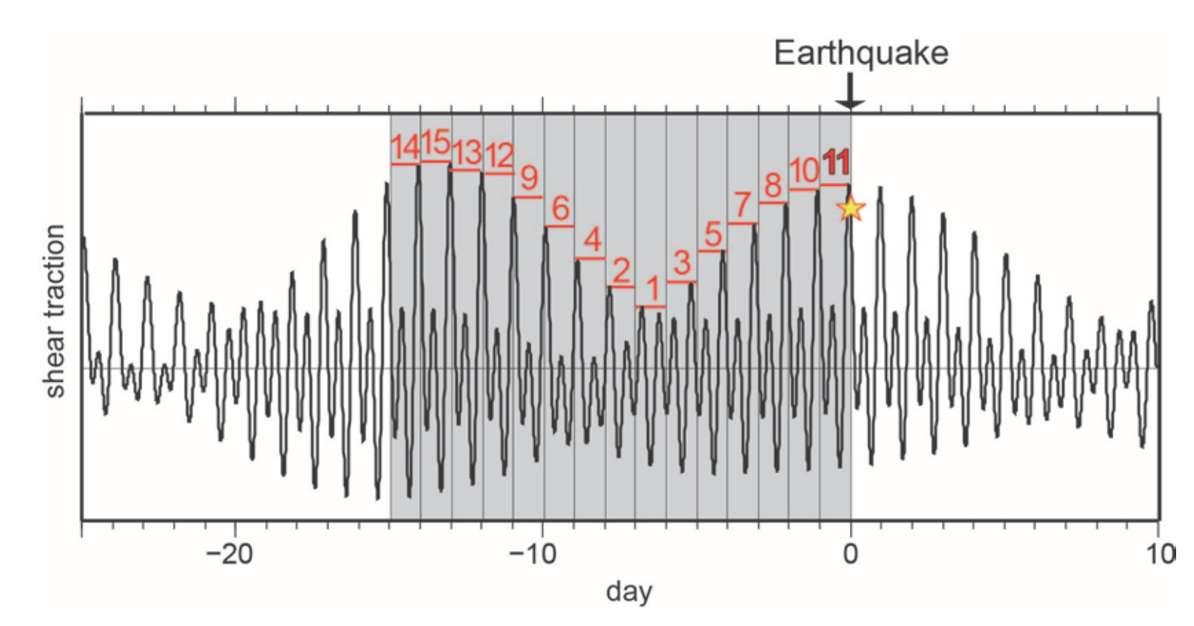
Cochran et al. estimated the background stress using a metric called τp, which is simply the average of the stress maxima occurring just before and just after each earthquake - the average of τpa and τpb in the figure below.

Figure 21: Diagram illustrating how to calculate τp. For an earthquake that occurred at the time of the star, find the values of τpa and τpb - the maxima on either side of the earthquake time, and take the average: τp = (τpa + τpb)/2. This can be done for any stress component (e.g., Δτ, Δσ, ΔCFF for any friction) . Figure 1 of Cochran et al. (2004).

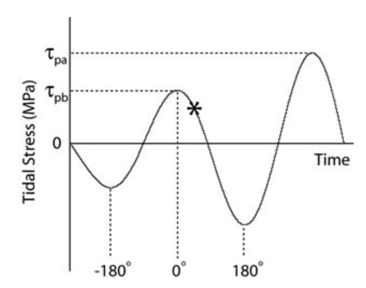
They counted how many earthquakes occurred during tidal phases that should drive failure (-90° < phase < 90°), compared to the expectation from uniform sampling. This value, called Nex, is the excess number of events during encouraging phases. Nex should be 0 on average, for random tidal phases.

Finally, they looked at the probability of finding at least Nex events out of a dataset of N events, if the events were random. Because phases are separated evenly into driving and resisting categories, this is the same as flipping a fair coin N times - a bi “two” nomial “term“ probability distribution. (You can simulate a series of coin flips and then calculate the binomial probability with this calculator - the binomial probability is the “at least” category.)

Because they expected a bigger effect for higher τp, they sorted their earthquake catalog from largest τp to smallest τp, and calculated the Nex and binomial probability for the growing set of N earthquakes, adding in one earthquake at a time. The result is the set of curves shown below. The first curve simply shows the accrual of excess events. The second curve shows the probability of finding that number of excess events, given N samples. Where the curve drops down toward values of 0%, there have been an unusual number of excess events.

Figure 22: Figures 3B,D of Cochran et al. Earthquakes are sorted by τp (largest to smallest), and the binomial probability of excess events is calculated for the subset of earthquakes up to N. Our red arrow annotates that N (with associated statistics) that was selected for reporting in the text.

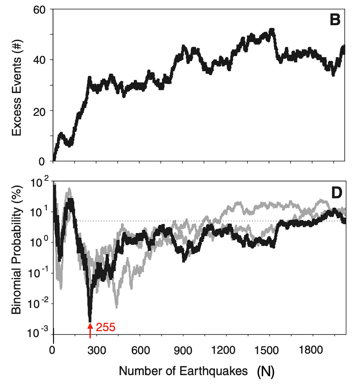
For the top 255 earthquakes with high τp, there were a lot of excess events - so many that the probability of finding that number randomly was only 0.0027%. As they added in more events with lower τp, however, the probability increased - the effect became less pronounced. Cochran et al. concluded that only the most highly stressed faults were responsible for the signal, which was then diluted as they added in less-stressed faults. However, the curve is a bit complex, and they noted that the first 45 events were strongly correlated; the next 100 were not as highly correlated; and the following 100 events were again strongly correlated, with a minimum binomial probability at N=255.

OK - we know what to look for, so let’s replicate the study.

First, we matched our data selection to Cochran et al. as best we could: using centroid locations, for 1977 through 2000 (inclusive), for thrust earthquakes M5.5+ above 40 km depth. Cochran et al.’s selection resulted in 2027 events; we found 2178 events. Our working catalog should include the events used by Cochran et al., plus an additional ~5% of events. We calculated τp for all phases and both nodal planes (available at GitHub), but here we will only talk about ΔCFF0.4 on the lower-dip nodal plane, which is what the paper focuses on.

So, what did we find?

Figure 23: Replication of Cochran et al.’s Figure 3B,D for pre-2001 earthquakes at centroid location, ΔCFF0.4.

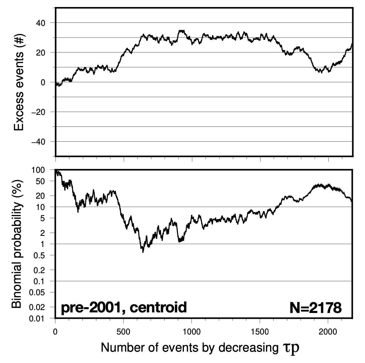
Our curve is similar to the published curve, although not exactly the same. As we progressively add events to our pile, starting with the highest τp and moving to lower values, the number of excess events does steadily increase. The corresponding binomial probability drops steeply at first, then rises slowly, and then drops again. Our minimum probability occurs at N=643, where we find a binomial probability of 0.58% - a “statistically meaningful” number, although larger than the minimum of Cochran et al. After that, the number of excess events stays flat for about 1000 events, and the binomial probability slowly rises back toward higher values.

This behavior is close enough to the results of Cochran et al. (2004) that we believe it counts as a validation of their calculations. In fact, the signal might be “better,” because we don’t see such wild (and hard to explain) swings in binomial probability at high τp.

Why don’t we replicate their exact curve? There seem to be several factors at play.

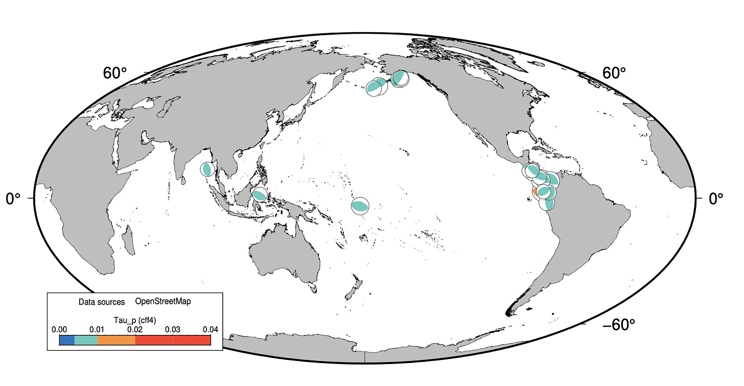
First, our estimated τp values are much smaller. While Cochran et al. found 19 shallow thrust events with τp above 0.02 MPa (with a maximum ~0.045 MPa) and another 41 events with τp between 0.01 and 0.02 MPa, our maximum τp only reached 0.011 MPa for shallow thrust earthquakes over the same time period, for the same stress type.

Are our calculations wrong? We compared our tidal calculations to those of Ide et al. (2016), who provided 60-day curves for tidal shear stress for fifteen specific earthquakes using a different calculation approach and tidal model. Our estimates closely match theirs. So, we think our values are probably good.

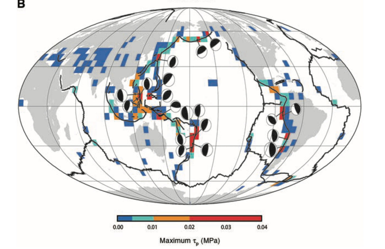
Second, our very highest stress earthquakes are not the same ones discovered by Cochran et al. Their 19 most highly stressed events (τp>=0.02 MPa) are distributed around the Pacific Rim, with many events in Tonga and offshore of Chile. These events are indicated by the focal mechanisms on their Figure 2B:

Figure 24: Figure 2B of Cochran et al. (2004), showing the areas where they find highest values of τp, for ΔCFF0.4.

When we plotted our own 19 most highly stressed earthquakes, the distribution was different. Our events are more concentrated in specific regions. Why would that be?

Figure 25: The 19 events with highest τp in our catalog, for shallow thrust events at centroid locations, ΔCFF0.4.

Since the magnitude of τp should depend mainly on the amount of ocean loading, which is directly related to tidal range, we thought this might be due to patterns of ocean tides. To evaluate this, we sought out a raster of lowest astronomical tide compared to mean sea level (Poncelet et al., 2021). This dataset represents approximately half of the full tidal range - where the values are strongly negative, the sea level reaches significant lows due solely to tides, over the course of about 20 years. (While it would be great to have a raster of highest astronomical tide, we couldn’t find or make one ourselves.)

On the maps below, the brown areas show where tides should also get high - where tidal stresses should reach large values, and τp values should also be high. On these maps, we plotted focal mechanisms of our 50 highest τp earthquakes in our replication dataset (pre-2001). You can see that they all occur in brown areas - regions of high tidal range.

Figure 26: Map of lowest astronomical tide from Poncelet et al. (2021). Focal mechanisms for our 50 highest τp earthquakes in our replication dataset (centroids, pre-2001, ΔCFF0.4) are plotted, colored and sized by τp.

Figure 27: Map of lowest astronomical tide from Poncelet et al. (2021). Focal mechanisms for our 50 highest τp earthquakes in our test dataset (centroids, post-2001, ΔCFF0.4) are plotted, colored and sized by τp.

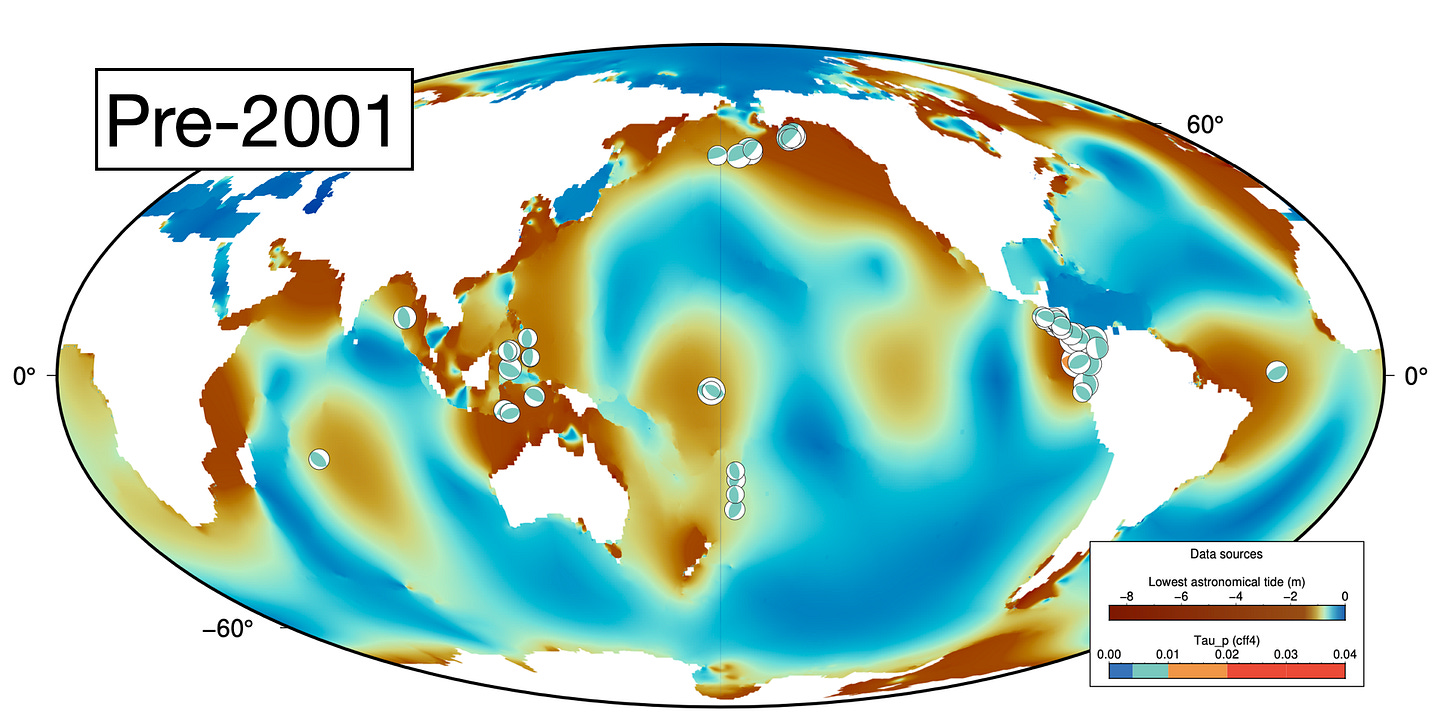
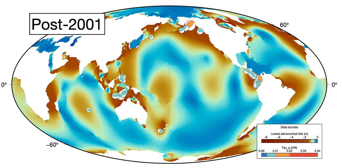
We sampled the lowest astronomical tide raster at event locations from the full GCMT catalog, discarding sites on land. We plotted the data to show how τp (y-axis) depends on both earthquake depth (x-axis) and on tidal range (color, brown = larger tidal range). The highest τp events occur only on the right side of the plot - they are shallow. This is because ocean tides are a surface load that diminishes in strength with depth. These high-τp events are also brown: they occur at locations with large tidal range. Many earthquakes in areas with large tidal range have low τp, because they occur at times when the fortnightly tides are low. Thus, for an earthquake to fall into our high-τp bin, it must (1) be located in an area with large tidal range, (2) occur at shallow depth, and (3) occur at a time when the fortnightly tide is high.

Figure 28: Plot of τp (for centroids, ΔCFF0.4) vs. depth for all earthquakes in the GCMT catalog below the oceans. Earthquakes are colored by lowest astronomical tide at their latitude and longitude; brown = larger tidal range.

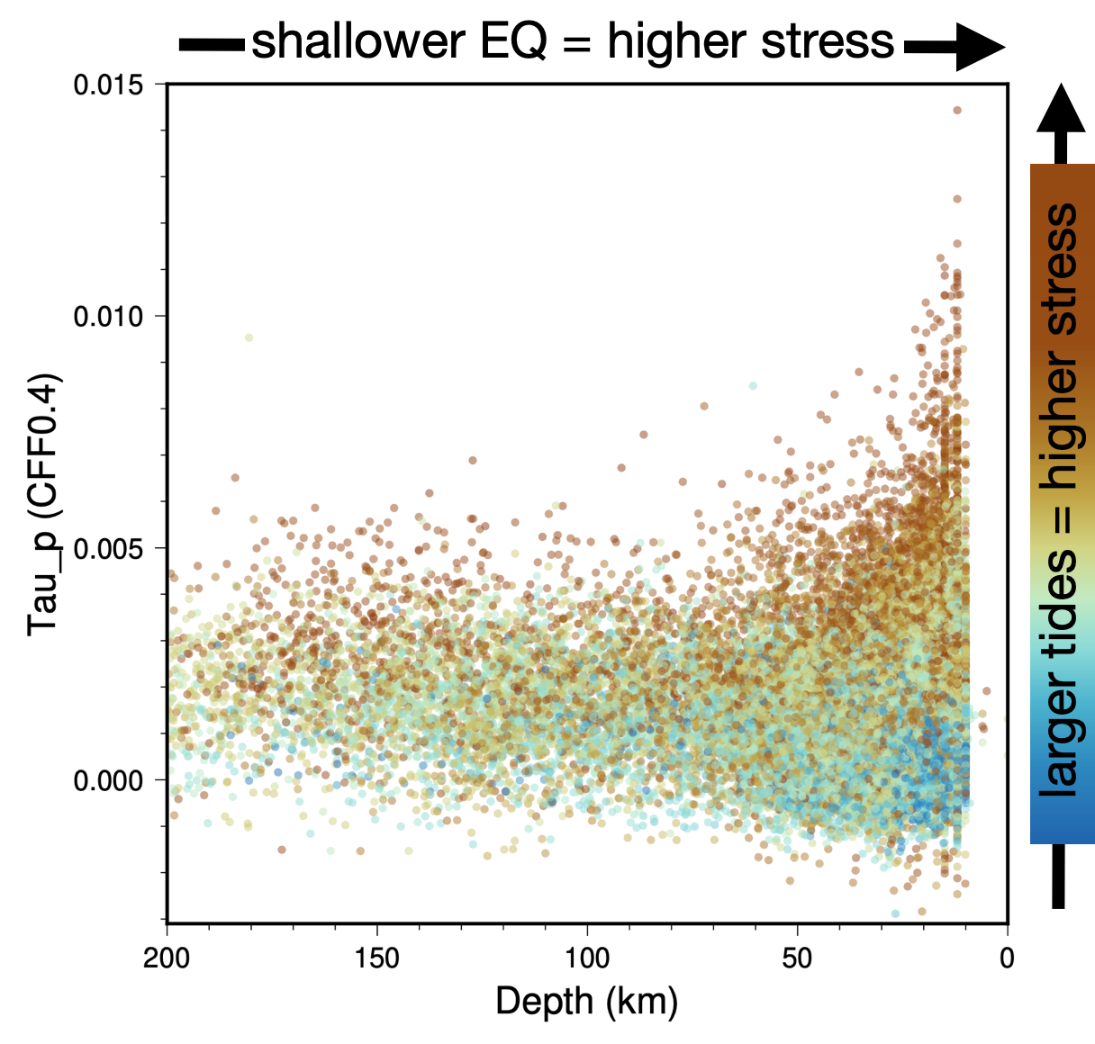
The clear dependence of τp on earthquake location and depth raises a further concern - which we have discussed before. Like Tanaka et al. (2002), Cochran et al. calculate tidal stresses at centroid locations, which can be significantly biased away from origin locations.

So, we wanted to test two things.

• First, does the result hold up when we use an independent dataset of earthquakes - those that occurred after 2001?

• Second, does the result hold up when we use origin locations for both the pre-2001 and post-2001 datasets?

The first test is pretty easy. We simply repeated our previous calculation, but for the independent dataset of post-2001 earthquakes. What do we see?

Figure 29: Our version of Cochran et al.’s Figure 3B,D for post-2001 earthquakes at centroid location, ΔCFF0.4.

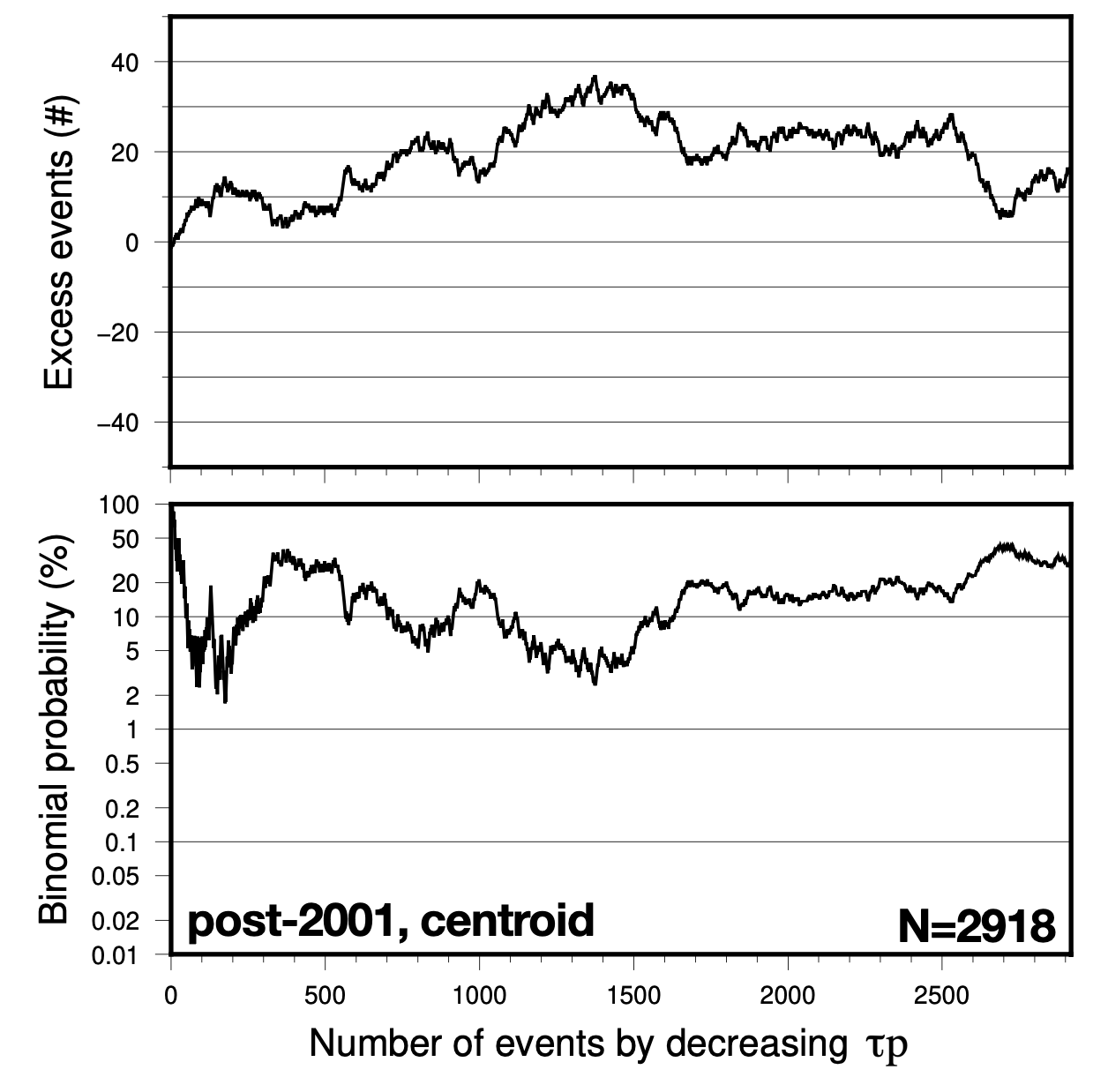
Well, we do see excess events that climb in number as we add high stress events, and we see an initial dip in the probability curve. However, the curve suggests that only the top 175 events have significant excess events, and we reach a minimum of 1.70%, which is not very compelling. After adding only about 10 excess events, we see a regression toward 0 and a lifting of the probability curve back above 20%. This wouldn’t be considered a strong result if we didn’t already know about the pre-2001 data.

Next, we performed the calculation on origin locations, for both the validation and testing time ranges. Here are the results:

Figure 30: Versions of Cochran et al.’s Figure 3B,D for pre-2001 earthquakes at origin locations (left) and post-2001 earthquakes at origin locations (right). ΔCFF0.4.

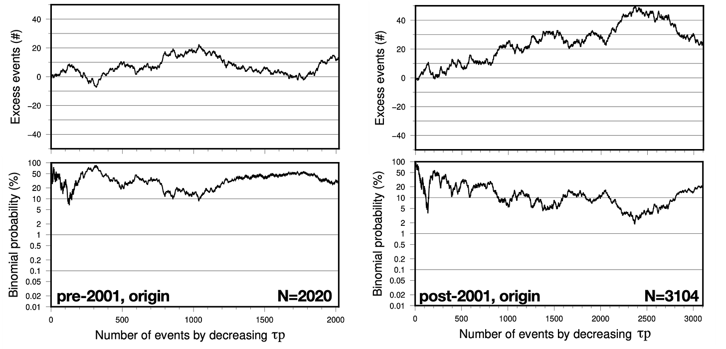
Both probability curves do have a small initial dip corresponding to about 10 excess events over about 120 earthquakes. Then, they both reverse back up to high probabilities over the next several hundred earthquakes, and then follow a zig-zaggy path.

These plots are not very compelling. It is important to note that binomial probability will have large swings at low N, which damp down as we add more events to our pile.

For fun, let’s plot a few binomial probability curves when the data are sorted using other factors, like latitude, date, depth, strike, and earthquake magnitude. These plots should give us a sense of what the same data pool produces for factors that we aren’t really willing to interpret physically.

Figure 31: Binomial probabilities for N earthquakes post-2001 shallow thrust earthquakes, M5.5+, sorted by (top left) decreasing latitude, (top right) decreasing date, (middle left) increasing depth, (middle right) decreasing strike, (bottom left) increasing magnitude, and (bottom right) increasing strike. Origin locations, ΔCFF0.4.

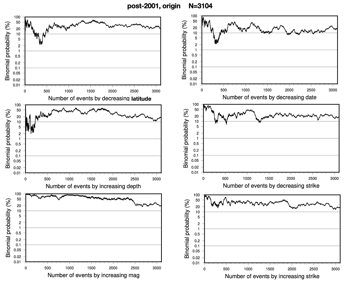
The curves all end up at the same point, since they all encapsulate the same overall dataset - just with different ordering. We sometimes see large fluctuations at low N, and they sometimes sink to relatively low probabilities (~2%). The charts don’t look that different than the original one, sorted by decreasing τp.

Finally, what if we just look at the full catalog, from 1977 to 2024, for both centroid and origin locations? This is the biggest and best dataset, after all.

Figure 32: Binomial probabilities for shallow thrust M5.5+ earthquakes from 1977-2024 sorted by τp (ΔCFF0.4), at (top) centroid and (bottom) origin locations.

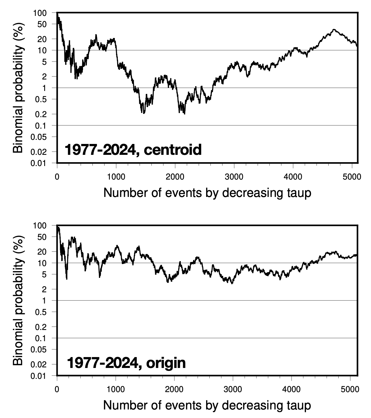
The curves are clearly different from each other - and while the centroid probabilities drop to nearly 0.2%, the origin probabilities remain at least an order of magnitude higher. We will discuss the origin-centroid issue at greater length in…. a future summary post. Sigh.

It is important to try to retain some perspective. We are only able to work with the earthquakes that have been observed - the statistics have already been decided. Out of 5096 earthquakes, the centroid location ΔCFF0.4 data have 40 excess events - a pretty small number. If the underlying process were random, we would achieve this number 13.4% of the time. For the origin location data, the number is 14.7% (38 excess events out of 5124 earthquakes).

In all of our plots of excess events, we see that the number of excess events doesn’t appear to climb faster at high τp than at lower τp ranges. So, it is hard to say that high τp events are special in any way. However, it’s true that the excess event number is not negative!

To sum up, while we do replicate the general pattern proposed in the study for pre-2001 data, the effect diminishes significantly in post-2001 data. Furthermore, it is clear that the centroid vs. origin problem is extremely important for this study - when origin locations are used, the effect basically disappears.

So, we think that we can’t reject the null hypothesis (that the catalog is random), either for the full catalog or for subsets with high τp.

Making sense of some funny histograms in Ide et al. (2016)

Hough (2018) already showed that the result of Ide et al. for only M8+ earthquakes is not replicable with a larger historical dataset. To end our post, we briefly discuss the interesting but confusing metric of tidal rank.

OK, you are to be commended if you made it this far. In case your spirit is flagging, in this section we don’t talk about anything revolutionary. We simply replicate a confusing (to us) distribution. So, feel free to skip ahead to the summary!

Anyway, over the course of our replications, we have learned that it is very important to try to understand the true distribution of tidal phases, tidal stresses, etc.

Let’s briefly consider an interesting and, to us, non-intuitive distribution. Ide et al. (2016) ranked earthquakes by comparing the maximum shear stress in the 24 hours before an earthquake to the same value over the two weeks prior. This is a fairly artificial metric, but it is intended to give a sense of when earthquake stresses are relatively high on average - kind of like τp, but over the two-week tidal cycle.

Figure 33: Ide et al.’s Supplementary Figure 2, showing an example of how to calculate the “stress ranking” of an earthquake.

Ide et al.’s stress rankings were plotted for four bins of earthquakes, each with a different magnitude cutoff.

Figure 34: Histograms of earthquakes for different magnitudes. Rankings reflect the position of the maximum Δτ on the day prior to the earthquake, compared to the fourteen days prior. Figure 2 of Ide et al. (2016).calculated a numerical ranking for earthquakes that relates the timing of the earthquake to the magnitude of peak stresses over the prior week. They showed that the tidal rank of most earthquakes - anything with magnitude less than 8.2, is no different than a random process.

For the fourth bin, representing the 11,397 earthquakes with Mw>5.5, they wrote:

The distribution in Fig. 2d is indistinguishable from the distribution made by random sampling of event timing.

We spent a lot of time puzzling over Figure 2d. Its shape - humped in the middle, with wings on either end - did not make sense to us. In our second post, we wrote:

Note: we don’t really understand, or rather really don’t understand, the shape of the histogram for all events (panel D). Ide et al. state that this is the shape we should expect for random events, but our intuition is that the histogram should be flat. We will investigate this further in future posts on this topic; any advice from the crowd is also welcome!

We don’t like not understanding things. So, we asked whether this distribution could be seen in a single tidal sea level curve (returning to our favorite location offshore Noto, Japan). After coding up the ranking algorithm, the distribution clearly emerged:

Figure 35: 60,000 samples of tidal rank for a 6-month period for a tidal sea level curve offshore Noto, Japan.

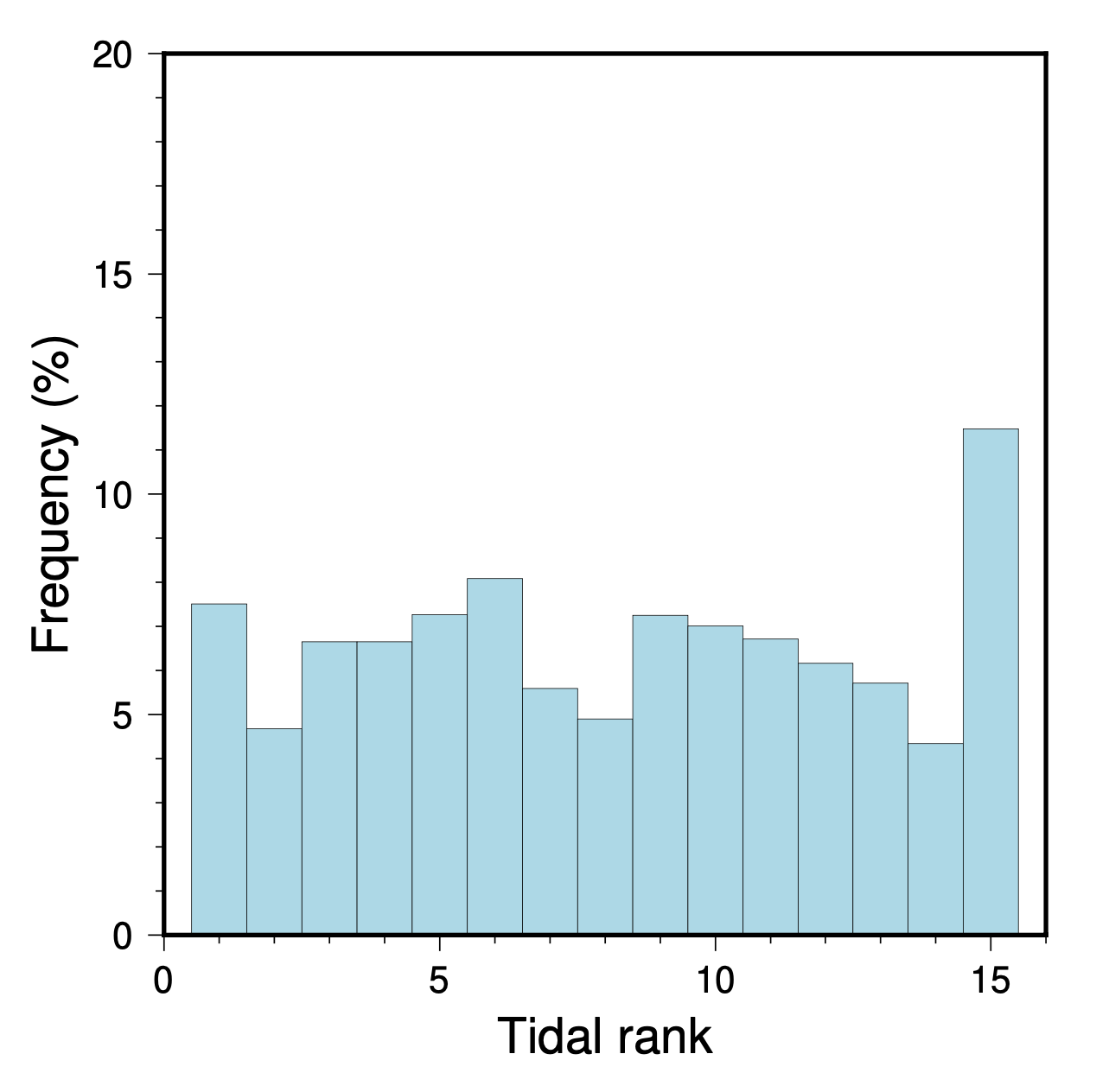
So, that just goes to show how intuition can be wrong. For the N=12 bin of largest-magnitude earthquakes, the theoretical distribution of ranks would probably be similar to, but not exactly the same as, a global average. In any case, it seems unlikely that such a small sample of 12 events could ever be interpreted meaningfully. Thus, we think that the primary conclusion of this part of Ide et al. (2016) is that the vast majority of earthquakes are not correlated with tidal rank.

Summing up

We tried our level best to replicate two important studies that proposed correlations between tides and earthquakes. In the end, we think we were able to replicate the methods well enough to test them appropriately, using data from more recent events and also using data at origin locations.

Our tests never showed as strong a signal as the original proposals. In some cases, the effect disappears entirely. In other cases, the results simply become too equivocal. A full exploration of the data beyond these direct tests might be interesting, but could also lead to unintentional p-hacking (the search for strong correlations in subsets of data).

Tanaka et al. (2002) warned about the dangers of subdivision…

… a prediction that seems to have borne out over 20 years of new data.

What’s next?

We just looked at global earthquakes covering almost 50 years - with significant difficulty.

One of the most promising fields of tidal earthquake triggering is based on the idea that faults might become more sensitive to tidal stresses as they approach failure. Some of the methods discussed in this post have already been applied to this problem - resulting in claims of clear tidal signals (tidalaciousness?) that heralded important earthquakes.

Because those studies have to subdivide datasets by time, they end up with very small N - between 20 and 100. Our suspicions are aroused.

So, in our next post, we will add the dimension of time. We will look at a series of papers that claim that they could have (possibly) foreseen some of Earth’s largest and most damaging earthquakes using tidal correlations - including the 2004 M9.1 Sumatra earthquake and the 2011 M9.3 Tohoku-Oki earthquake.

These kinds of claims tend to get a lot of attention, because if they were true, then there would be a strong chance that we could make some earthquake predictions…

Will these papers stand up to testing? Stay tuned for our next post to find out.

Open Data

Would you like to replicate our replications or validate our validations? We have uploaded the full GCMT catalog containing our estimated tidal phases, stress amplitudes, and τp values, for both nodal planes, for both centroid and origin locations, to GitHub:

https://github.com/kyleedwardbradley/tidal_gcmt

Please feel free to use these data in any way you wish. If you do some science, drop us a note!

Papers that should be credited when the data are used (GCMT, TidalStrain.2) are listed on the GitHub page.

References:

Bradley, K., Hubbard, J., 2024. The great tidal earthquake hypothesis test, part I. Earthquake Insights, https://doi.org/10.62481/9ab803be

Cochran, E.S., Vidale, J.E. and Tanaka, S., 2004. Earth tides can trigger shallow thrust fault earthquakes. Science, 306(5699), pp.1164-1166. https://doi.org/10.1126/science.1103961

Hirose, F., Maeda, K. and Kamigaichi, O., 2019. Tidal forcing of interplate earthquakes along the Tonga‐Kermadec Trench. Journal of Geophysical Research: Solid Earth, 124(10), pp.10498-10521. https://doi.org/10.1029/2019JB018088

Hirose, F., Maeda, K. and Kamigaichi, O., 2022. Efficiency of earthquake forecast models based on earth tidal correlation with background seismicity along the Tonga–Kermadec trench. Earth, Planets and Space, 74(1), pp.1-11. https://doi.org/10.1186/s40623-021-01564-4

Hough, S.E., 2018. Do large (magnitude≥ 8) global earthquakes occur on preferred days of the calendar year or lunar cycle?. Seismological Research Letters, 89(2A), pp.577-581. https://doi.org/10.1785/0220170154

Hubbard, J. and Bradley, K., 2024. The great tidal earthquake hypothesis test, part II. Earthquake Insights, https://doi.org/10.62481/2c56f873

Hubbard, J. and Bradley, K., 2024. M7.5 earthquake strikes western Japan, triggers tsunami. Earthquake Insights, https://doi.org/10.62481/e8bf9b2e

Ide, S., Yabe, S. and Tanaka, Y., 2016. Earthquake potential revealed by tidal influence on earthquake size–frequency statistics. Nature Geoscience, 9(11), pp.834-837. https://doi.org/10.1038/ngeo2796

Matsumoto, K., T. Sato, T. Takanezawa, and M. Ooe, 2001, GOTIC2: A program for computation of oceanic tidal loading effect, J. Geod. Soc. Japan, 47, 243-248. https://doi.org/10.11366/sokuchi1954.47.243

Núñez, P., Castanedo, S. and Medina, R., 2020. A global classification of astronomical tide asymmetry and periodicity using statistical and cluster analysis. Journal of Geophysical Research: Oceans, 125(8), p.e2020JC016143. https://doi.org/10.1029/2020JC016143

Poncelet, C., Billant G., Saunier A. (2021). Global estimated surfaces of Lowest Astronomical Tide (LAT) and Mean Sea Level (MSL). SEANOE. https://doi.org/10.17882/85408

Tanaka, S., Ohtake, M. and Sato, H., 2002. Evidence for tidal triggering of earthquakes as revealed from statistical analysis of global data. Journal of Geophysical Research: Solid Earth, 107(B10), pp.ESE-1. https://doi.org/10.1029/2001JB001577

Tsuruoka, H., Ohtake, M. and Sato, H., 1995. Statistical test of the tidal triggering of earthquakes: contribution of the ocean tide loading effect. Geophysical Journal International, 122(1), pp.183-194. https://doi.org/10.1111/j.1365-246X.1995.tb03546.x

Schuster, A., 1897. On lunar and solar periodicities of earthquakes. Proceedings of the Royal Society of London, 61(369-377), pp.455-465. https://doi.org/10.1098/rspl.1897.0060